
Authors: Priyadharshini Jayakumar, Shreya Ramesh
Introduction
Predictive maintenance has become a cornerstone of modern industrial operations, enabling organizations to anticipate equipment failures and reduce costly downtime. A central task in predictive maintenance is Remaining Useful Life (RUL) prediction, which estimates the number of operating cycles left before a machine fails. Accurately predicting RUL allows businesses to schedule timely maintenance, optimize resource allocation, and extend equipment lifespan.
In this blog, we present our journey of reproducing the dual-attention deep learning model proposed by Wang et al. (2025) for RUL prediction. By following the methodology described in their paper, we sought to validate their approach, evaluate its performance on the NASA C-MAPSS dataset, and understand the role of attention mechanisms in improving predictive accuracy and interpretability.
This detailed walkthrough not only presents the steps we took but also reflects on the challenges, lessons learned, and opportunities for future research. Our reproduction experiment serves as both a validation of the research and a guide for practitioners looking to implement similar predictive maintenance pipelines.
Background: Why RUL Prediction Is Challenging
RUL prediction is inherently complex due to several key challenges:
- Non-linear degradation patterns: Machines rarely degrade in a simple, linear fashion. Different sensors may capture different degradation signatures, requiring advanced modeling techniques.
- Variable operating conditions: Machines often operate under multiple regimes (e.g., varying loads, speeds, and environmental factors). A model must generalize across these conditions.
- Lack of early degradation signals: In the initial operating cycles, sensor readings may not show significant changes, making it hard to learn useful patterns.
- Need for interpretability: Industrial stakeholders demand not only accurate predictions but also an understanding of why the model makes certain predictions. Sensor-level insights are critical for trust and adoption.
These challenges motivate the use of dual-attention mechanisms, which help a model focus both on the most informative sensors (channel attention) and on the most critical time steps (self-attention).
Dataset: NASA’s C-MAPSS Simulator
We used the C-MAPSS (Commercial Modular Aero-Propulsion System Simulation) dataset, a widely used benchmark for RUL prediction. It simulates turbofan engine degradation under varying operating conditions and fault modes.
The dataset consists of four subsets:
- FD001: 1 operating condition, 1 fault mode.
- FD002: 6 operating conditions, 1 fault mode.
- FD003: 1 operating condition, 2 fault modes.
- FD004: 6 operating conditions, 2 fault modes.
For this study, we focused on FD002, which is more challenging than FD001 due to multiple operating conditions, while still being manageable in complexity.
Raw Data Shapes
- Training Set: 53,759 × 26
- Test Set: 33,991 × 26
- RUL Labels: 259 × 1
Each row corresponds to a single engine cycle, with 26 columns, including unit identifiers, operating conditions, and 21 sensor readings.
Data Preprocessing
Before training, significant preprocessing was required to clean and structure the data for deep learning.
1. Sensor Selection
Not all sensors contribute meaningful degradation information. Based on prior literature and exploratory analysis, we removed the following non-degrading sensors:
- Sensors 1, 5, 6, 10, 16, 18, and 19
This left us with 14 informative sensors.
2. Normalization
To ensure stable training, we applied min–max scaling to all sensor values. Unit numbers and RUL labels were excluded from normalization.
3. RUL Clipping
Since extremely large RUL values can dominate the loss function without being practically useful, we clipped the maximum RUL to 125 cycles. The reasoning behind this is that, in the early life of an engine, when the true RUL is very large, it is not critical to know whether the remaining life is 200 cycles, 300 cycles, or even more. From a maintenance perspective, the engine is still considered “healthy”, and the exact number of cycles left is less important.
What matters most is the model’s ability to accurately capture the degradation phase, i.e., when the engine approaches its failure window. By capping the maximum RUL, we prevent the model from wasting capacity by trying to learn distinctions that are irrelevant in practice (such as 280 vs. 310 cycles) and instead encourage it to focus on the region where predictive accuracy has the highest operational value.
This clipping technique is widely used in RUL prediction research and has been shown to stabilize training and improve the practical utility of the predictions.
4. Sliding Windows
Deep learning models require fixed-length sequences as input. To achieve this, we applied a sliding window of length 60 cycles with a stride of 1. Each training sample, therefore, consists of 60 time steps × 18 sensors.
- Number of test windows generated: 19,290
- Final test data shape: 19,290 × 60 × 18
One caveat of this approach is that engines with fewer than 60 cycles cannot form a complete window. Such engines were dropped from the dataset during preprocessing. This is a common trade-off in sequence modeling: by enforcing a fixed input length, we lose a few very short sequences, but ensure that the model can learn consistent temporal patterns across engines.
Model Architecture: Dual Attention
The dual-attention model combines two complementary mechanisms to improve RUL prediction:
1. CNN-CAM (Channel Attention Module)
- A 1D CNN processes sensor signals to extract local features.
- Channel attention weights sensors differently, allowing the model to focus on the most critical ones for degradation.
- Example: Temperature or vibration sensors may be more relevant than others.
2. GRU-SAM (Self-Attention Module)
- A GRU (Gated Recurrent Unit) layer captures temporal dependencies across 60 time steps.
- A self-attention mechanism highlights which time steps are most important for predicting degradation.
- Example: The final cycles before failure often carry stronger degradation signals.
3. Regression Head
- Fully connected layers map the extracted features into a scalar RUL prediction.
- Structure: [50, 10] hidden units with dropout.
This combination enables the model to balance both sensor-level and temporal-level interpretability.
4. Gradient Clipping
- Gradient clipping was applied with a maximum norm of 5 to stabilize training.
- This prevents exploding gradients during backpropagation, improving convergence stability, particularly in the GRU layers.
Training Setup
We configured the training based on the paper’s specifications:
- Convolutional kernels: 4
- Kernel size: 1 × 3
- CNN activation: tanh
- GRU hidden units: 50
- GRU activation: ReLU
- Fully connected layers: [50, 10]
- Dropout: 0.2
- Learning rate: 0.001
- Optimizer: Adam
- Epochs: 30
- Batch size: 64
- Window size: 60
Training converged stably, with validation losses decreasing consistently.
Results
On the FD002 test set, our reproduction delivered strong performance:
- MAE (Mean Absolute Error): 11.15 → On average, the model’s predictions were off by only about 11 cycles, which is quite precise, given the complexity of the task.
- RMSE (Root Mean Square Error): 15.35 → Large errors were well controlled, with no drastic prediction failures.
- R² (Coefficient of Determination): 0.866 → The model explains nearly 87% of the variance in the true RUL values, a strong indicator of predictive reliability.
Although gradient clipping was not used in the original paper, our implementation helped stabilize GRU training, reducing large fluctuations and slightly improving validation performance.
What makes these results exciting is not just the raw numbers, but the consistency with the original paper’s findings. Our reproduction validates the effectiveness of the dual-attention mechanism: CNN-CAM successfully highlights the most relevant sensors, while GRU-SAM captures critical temporal patterns. In practice, this means the model can tell when the engine is approaching failure and which sensors provide the clearest warning signs.
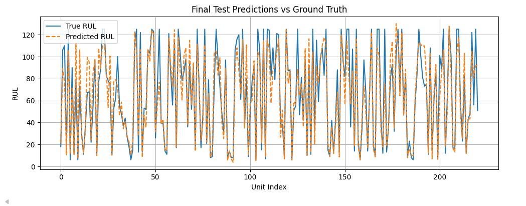
To further illustrate model performance, the following figure compares predicted RUL values against ground-truth labels for all engines in the FD002 test set. The close alignment between the blue (true RUL) and orange (predicted RUL) lines highlights the accuracy of the model.
Evaluation Metrics
We evaluated the model using three widely accepted metrics:
- Root Mean Square Error (RMSE) – Penalizes large errors more heavily.
- Mean Absolute Error (MAE) – Captures the average deviation from true RUL.
- R² (Coefficient of Determination) – Measures goodness of fit; values closer to 1 indicate better predictive accuracy.
Together, these metrics provide a comprehensive view of model performance.
Explainability with Captum
Interpretability is crucial for industrial applications. We used Captum, a PyTorch library for model explainability.
Global Importance – Integrated Gradients
One of the key extensions we added beyond the original paper was model interpretation. Using Captum’s Integrated Gradients, we quantified the contribution of each sensor to the RUL predictions.
The bar chart below shows the global feature importance, averaged across the dataset:
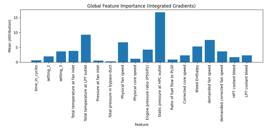
Several interesting insights emerged:
- Static pressure at the HPC outlet dominated feature importance, confirming its strong correlation with engine degradation.
- Total temperature at the LPT outlet and physical fan speed were also among the top contributors.
- Many less-informative sensors (e.g., bypass duct pressure, cycle count) contributed minimally, which validates our earlier sensor selection step.
This interpretation step adds an extra layer of confidence: the model isn’t just performing well numerically — it is relying on sensors that align with domain knowledge about turbofan engine physics. This kind of interpretability is crucial for real-world deployment, where maintenance engineers need to understand why a model is making a prediction.
Local Importance – Saliency Maps
In addition to global analysis, we also examined local explanations for individual engines. Using Saliency Maps, we evaluated which sensors had the strongest influence on a specific prediction.
The plot below shows saliency for Sample #100, averaged across its 60 time steps:
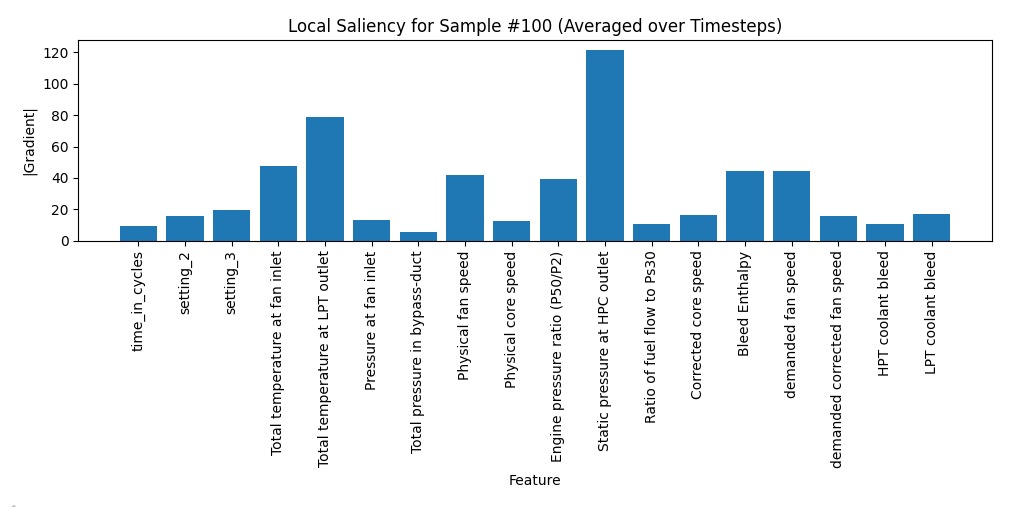
Key Observations:
- Static pressure at the HPC outlet again emerged as the dominant factor, consistent with global analysis.
- Total temperature at the LPT outlet and physical fan speed also contributed strongly.
- Less relevant sensors, such as bypass duct pressure, had minimal influence.
Interestingly, when repeating this analysis for multiple engines, we found that the same set of sensors consistently dominated predictions. This consistency suggests that the model’s learned representations are robust and not overly dependent on noise or random correlations.
This step demonstrates that the model is not only accurate but also trustworthy and interpretable — a crucial requirement for adoption in real-world predictive maintenance systems.
Lessons Learned
From reproducing this model, we gained several key insights:
- Sensor selection is crucial – Removing non-degrading sensors improves performance.
- RUL clipping stabilizes training – Prevents extreme values from distorting learning.
- CAM contributes more than SAM – Sensor-level attention had a stronger impact on performance.
- Captum confirmed interpretability – Consistent explanations build trust in real-world use cases.
Future Work
While the dual-attention approach is promising, there are several avenues for extension:
- Transfer Learning: Apply knowledge across FD001–FD004 datasets.
- Lightweight Deployment: Optimize the model for edge devices in industrial settings.
- Transformer Models: Explore Transformer-based architectures for long-sequence modeling.
- Temporal Attribution: Develop advanced visualization methods for time-based feature importance.
- Domain-Guided Feature Emphasis: Beyond purely data-driven attention mechanisms, we plan to explore ways to embed domain knowledge into the model. For example, if aerospace engineers already know that static pressure at the HPC outlet or LPT temperature are critical degradation indicators, the model can be guided to emphasize these columns explicitly during training. This hybrid of data-driven learning and expert knowledge could improve both accuracy and trustworthiness.
Conclusion
By reproducing the work of Wang et al. (2025), we validated the effectiveness of their dual-attention RUL prediction model. The combination of CNN-CAM (channel attention) and GRU-SAM (self-attention) achieved strong predictive accuracy while maintaining interpretability. Our results underscore the importance of both sensor-level and temporal-level attention in predictive maintenance.
This work not only reinforces the findings of the original research but also provides a practical blueprint for building robust predictive maintenance pipelines. With further improvements in transfer learning and lightweight deployment, such models can play a transformative role in modern industry.
References
Wang, Fan, et al. “A deep-learning method for remaining useful life prediction of power machinery via dual-attention mechanism.” Sensors, vol. 25, no. 2, 2025, p. 497. MDPI, https://doi.org/10.3390/s25020497.
